9 Loss, optimization, and regularization
This chapter covers
- Geometrical and algebraic introductions to loss functions
- Geometrical intuitions for softmax
- Optimization techniques including momentum, Nesterov, AdaGrad, Adam, and SGD
- Regularization and its relationship to Bayesian approaches
- Overfitting while training, and dropout
By now, it should be etched in your mind that neural networks are essentially function approximators. In particular, neural network classifiers model the decision boundaries between the classes in the feature space (a space where every input feature combination is a specific point). Supervised classifiers mark sample training data inputs in this space with a—perhaps manually generated—class label (ground truth). The training process iteratively learns a function that essentially creates decision boundaries separating the sampled training data points into individual classes. If the training data set is a reasonable representative of the true distribution of possible inputs, the network (the learned function that models the class boundaries) will classify never-before-seen inputs with good accuracy.
When we select a specific neural network architecture (with a fixed set of layers, each with a fixed set of perceptrons with specific connections), we have essentially frozen the family of functions we use as a function approximator. We still have to “learn” the exact weights of the connectors between various perceptrons aka neurons). The training process iteratively sets these weights so as to best classify the training data points. To do this, we design a loss function that measures the departure of the network output from the desired result. The network continually tries to minimize this loss. There are a variety of loss functions to choose from.
The iterative process through which loss is minimized is called optimization. We also have a multitude of optimization algorithms to choose from. In this chapter, we study loss functions, optimization algorithms, and associated topics like L1 and L2 regularization and dropout. We also learn about overfitting, a potential pitfall to avoid while training a neural network.
NOTE The complete PyTorch code for this chapter is available at http://mng.bz/aZv9 in the form of fully functional and executable Jupyter notebooks.
9.1 Loss functions
A loss function essentially measures the badness of the neural network output. In the case of a supervised network, the loss for an individual training data instance is the distance of the actual output of the neural network (aka prediction) from the desired ideal outputs known or manually labeled ground truth [GT]) on that particular training input instance. Total training loss is obtained by summing the losses from all training data instances. Training is essentially an iterative optimization process that minimizes the total training loss.
9.1.1 Quantification and geometrical view of loss
Loss surfaces and their minimization are described in detail in section 8.4.2. Here we only do a quick review.
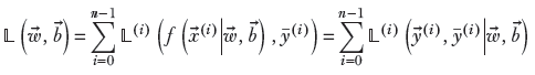
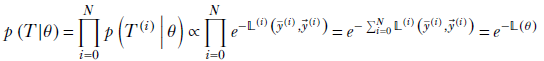
A full neural network can be described by the equation
![]()
Equation 9.1
Equation 9.1 says that given an input ![]() , the neural network with weights
, the neural network with weights ![]() and biases
and biases ![]() emits the output vector or prediction vector
emits the output vector or prediction vector ![]() . The weights and biases may be organized into layers; this equation does not care. The vectors
. The weights and biases may be organized into layers; this equation does not care. The vectors ![]() ,
, ![]() , respectively, denote the sets of all weights and biases from all layers aggregated. Evaluating the function f(⋅) is equivalent to performing one forward pass on the network. In particular, given a training input instance
, respectively, denote the sets of all weights and biases from all layers aggregated. Evaluating the function f(⋅) is equivalent to performing one forward pass on the network. In particular, given a training input instance ![]() (i), the neural network emits
(i), the neural network emits ![]() (i) = f(
(i) = f(![]() (i)|
(i)|![]() ,
, ![]() ). We refer to
). We refer to ![]() (i) as the output of the ith training data instance.
(i) as the output of the ith training data instance.
During supervised training, for each training input instance ![]() (i), we have the GT (the known output), ȳ(i). We refer to ȳ(i) as the GT vector (as usual, we use superscript indices for training data instances).
(i), we have the GT (the known output), ȳ(i). We refer to ȳ(i) as the GT vector (as usual, we use superscript indices for training data instances).
Ideally, the output vector ![]() (i) should match the GT vector ȳ(i). The mismatch between them is the loss for that training data instance 𝕃(i)(
(i) should match the GT vector ȳ(i). The mismatch between them is the loss for that training data instance 𝕃(i)(![]() (i), ȳ(i)|
(i), ȳ(i)|![]() ,
, ![]() ), which we sometimes denote as 𝕃(i)(
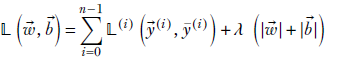
), which we sometimes denote as 𝕃(i)(![]() (i), ȳ(i)). The overall training loss (to be minimized by the optimization process) is the sum of losses over all training data instances:
(i), ȳ(i)). The overall training loss (to be minimized by the optimization process) is the sum of losses over all training data instances:
Equation 9.2
where the summation is over all training data instances, and n is the size of the training data set. Note that this summation over all training data points is needed to compute the loss for each training data instance. Thus an epoch, a single training loop over all training data instances, costs O(n2), where n is the number of training data points. Training usually requires many epochs. This makes the training process very expensive. In section 9.2.2, we study ways of mitigating this.
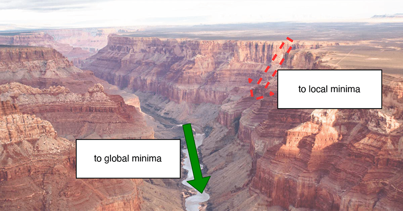
Figure 9.1 The loss surface can be viewed as a canyon.
NOTE In this chapter, we use n to indicate the number of training data points and N to indicate the dimensionality of the output vector. For classifiers, the dimensionality of the output vector, N, matches the number of classes. We also use superscript (i) to index training data points and subscript j to index output vector dimensions. For classifiers, j indicates the class.
We can visualize 𝕃(![]() ,
, ![]() ) as a hypersurface in high-dimensional space. Figures 8.8 and 8.9 show some low-dimensional examples of loss surfaces. These are illustrative examples. In reality, the loss surface is typically high dimensional and very complex. One good mental picture is that of a canyon (see figure 9.1). Traveling “downhill” at any point effectively follows the negative direction of the local gradient the gradient of a loss surface was introduced in section 8.4.2). Traveling downhill along the gradient does not always lead to the global minimum. For instance, going downhill following the dashed arrow will take us to a local minimum, whereas the global minimum is where the water is going, indicated by the solid arrow. (See also section 8.4.4 and figure 8.9.)
) as a hypersurface in high-dimensional space. Figures 8.8 and 8.9 show some low-dimensional examples of loss surfaces. These are illustrative examples. In reality, the loss surface is typically high dimensional and very complex. One good mental picture is that of a canyon (see figure 9.1). Traveling “downhill” at any point effectively follows the negative direction of the local gradient the gradient of a loss surface was introduced in section 8.4.2). Traveling downhill along the gradient does not always lead to the global minimum. For instance, going downhill following the dashed arrow will take us to a local minimum, whereas the global minimum is where the water is going, indicated by the solid arrow. (See also section 8.4.4 and figure 8.9.)
Many loss formulations are possible, quantifying the mismatch 𝕃(i)(![]() (i), ȳ(i)); some of them are described in the following subsections.
(i), ȳ(i)); some of them are described in the following subsections.
9.1.2 Regression loss
Regression loss is the simplest loss formulation. It is the L2 norm of the difference between the output and GT vectors. This loss was introduced in equation 8.11. We restate it here: the loss on the ith training data instance is
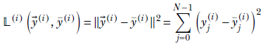
where the summation is over the components of the output vector. N is the number of classes. The GT vector and output vector are both N-dimensional.
NOTE Fully functional code for regression loss, executable via Jupyter Notebook, can be found at http://mng.bz/g1a8.
Listing 9.1 PyTorch code for regression loss
from torch.nn.functional import mse_loss                   ①

y_pred = torch.tensor([-0.10, -0.24,  1.43, -0.14, -0.59]) ②

y_gt = torch.tensor([ 0.59, -1.92, -1.27, -0.40,  0.50])   ③

loss = mse_loss(y_pred, y_gt, reduction='sum')             ④
① Imports the regression loss (mean squared error loss)
② N-d prediction vector
③ N-d ground truth vector
④ Computes the regression loss
9.1.3 Cross-entropy loss
Cross-entropy loss was discussed in the context of entropy in section 6.3. If necessary, this would be a great time to reread that. Here we review the idea quickly.
Cross-entropy loss is typically used to measure the mismatch between a classifier neural network output and the corresponding GT in a classification problem. Here, the GT is a one-hot vector whose length equals the number of classes. All but one of its elements are 0. The single nonzero element is 1, and it occurs at the index corresponding to the correct class for that training data instance.
Thus the GT vector looks like ȳ(i) = [0,…,0,1,0,…,0]. The prediction vector should have elements with values between 0 and 1. Each element of the prediction vector ![]() (i) indicates the probability of a specific class. In other words,
(i) indicates the probability of a specific class. In other words, ![]() (i) = [p0, p1,…, pN−1], where pj is the probability of the input i belonging to the jth class. In section 6.3, we illustrated with an example image classifier that predicts whether an image contains a cat class 0), a dog (class 1), an airplane (class 2), or an automobile (class 3). One of the four is always assumed to be present in the image. If, for the ith training data instance, the GT vector is an image of cat, we have ȳ(i) = [1,0,0,0]. A prediction vector
(i) = [p0, p1,…, pN−1], where pj is the probability of the input i belonging to the jth class. In section 6.3, we illustrated with an example image classifier that predicts whether an image contains a cat class 0), a dog (class 1), an airplane (class 2), or an automobile (class 3). One of the four is always assumed to be present in the image. If, for the ith training data instance, the GT vector is an image of cat, we have ȳ(i) = [1,0,0,0]. A prediction vector ![]() (i) = [0.8,0.15,0.04,0.01] is good, while
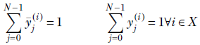
(i) = [0.8,0.15,0.04,0.01] is good, while ![]() (i) = [0.25,0.25,0.25,0.25] is bad. Note that sum of the elements of the GT as well as the prediction vector is always 1 since they are probabilities. Mathematically, given a training dataset X,
(i) = [0.25,0.25,0.25,0.25] is bad. Note that sum of the elements of the GT as well as the prediction vector is always 1 since they are probabilities. Mathematically, given a training dataset X,
Given such GT and prediction vectors, the cross-entropy loss (CE loss) is
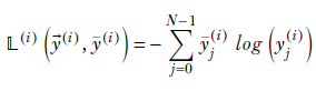
Equation 9.3
where the summation is over the elements of the prediction vector and N is the number of classes.
Intuitions behind cross-entropy loss
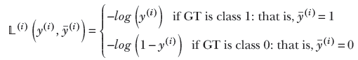
Note that only one element—the one corresponding to the GT class—survives in the summation of equation 9.3. The other elements vanish because they are multiplied by the 0 GT value. The (logarithm of) the predicted probability of the correct GT class is multiplied by 1. Hence, the CE loss always boils down to −log(yj*(i)), where j* is the GT class. If this probability is 1, the CE loss becomes 0, rightly so, as the correct class is being predicted with a probability of 1. If the predicted probability of the correct class is 0, the CE loss is −log(0) = ∞, again rightly so, since this is the worst possible prediction. The closer the prediction for the correct class is to 1, the smaller the loss.
NOTE Fully functional code for cross-entropy loss, executable via Jupyter Notebook, can be found at http://mng.bz/g1a8.
Listing 9.2 PyTorch code for cross-entropy loss
import torch

y_pred = torch.tensor([0.8, 0.15, 0.04, 0.01]) ①

y_gt = torch.tensor([1., 0., 0., 0.])          ②

loss = -1 * torch.dot(y_gt, torch.log(y_pred)) ①
① N-d prediction vector
② N-d one-hot ground truth vector
③ Computes the cross-entropy loss
Special case of two classes
What happens if N = 2 (that is, we have only two classes)? Let’s denote the predicted probability of class 0, for the ith training input, as y(i): that is, ![]() 0(i) = y(i). Then, since these are probabilities, the prediction on the other class
0(i) = y(i). Then, since these are probabilities, the prediction on the other class ![]() 1(i) = 1 − y(i). Also, let ȳ(i) denote the GT probability for class 0 on this ith training input. Then 1 − ȳ(i) is the GT probability for class 1. (We have slightly abused notations—up to this point, ȳ has denoted a vector, but here it denotes a scalar.)
1(i) = 1 − y(i). Also, let ȳ(i) denote the GT probability for class 0 on this ith training input. Then 1 − ȳ(i) is the GT probability for class 1. (We have slightly abused notations—up to this point, ȳ has denoted a vector, but here it denotes a scalar.)
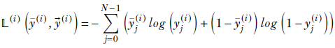
Then, following equation 9.3, the CE loss on the ith training data instance becomes
𝕃(i)(y(i), ȳ(i)) = −ȳ(i) log(y(i)) − (1−ȳ(i)) log(1−y(i))
Equation 9.4
NOTE Fully functional code for binary cross-entropy loss, executable via Jupyter Notebook, can be found at http://mng.bz/g1a8.
Listing 9.3 PyTorch code for binary cross-entropy loss
from torch.nn.functional import binary_cross_entropy ①

y_pred = torch.tensor([0.8])                         ②

y_gt = torch.tensor([1.])                            ③

loss = binary_cross_entropy(y_pred, y_gt)            ④
① Imports the binary cross-entropy loss
② Outputs the probability of class 0 - y0. A single value is sufficient because y1 = 1 − y0.
③ The ground truth is either 0 or 1.
④ Computes the cross-entropy loss
9.1.4 Binary cross-entropy loss for image and vector mismatches
Given a pair of normalized tensors (such as images or vectors) whose elements all have values between 0 and 1, a variant of the two-class CE loss can be used to estimate the mismatch between the tensors. Note that an image with pixel-intensity values between 0 and 255 can always be normalized by dividing each pixel-intensity value by 255, thereby converting it to the 0 to 1 range. Such a comparison of two images is used in image autoencoders, for example. We study autoencoders later; here, we provide a brief overview in the following sidebar.
Let ȳ denote the input image. Let ![]() (i) denote the reconstructed image outputted by the autoencoder. The binary cross-entropy loss is defined as
(i) denote the reconstructed image outputted by the autoencoder. The binary cross-entropy loss is defined as
Equation 9.5
Note that here N is the number of pixels in the image, not the number of classes, as before. The summation is over the pixels in the image. Also, the GT vector ȳ(i) is not a one-hot vector; rather, it is the input image. These differences aside, equation 9.5 is based on the same idea as equation 9.4.
Why does it work?
Binary cross-entropy loss attains its minimum when the input matches the GT. We outline the proof next. (Note that we drop the superscripts and subscripts for simplicity.) We have
−𝕃 = ȳlog(y) + (1 − ȳ)log(1 − y)
At the minimum, ∂𝕃/∂y = 0.
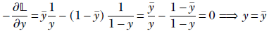
Thus, the minimum of the binary cross-entropy loss occurs when the network output matches the GT. However, this does not mean this loss becomes zero when the output matches the GT.
NOTE Binary cross-entropy loss is not necessarily zero even in the ideal case of the output matching the input (although the loss is indeed minimal in the ideal case, meaning the loss is higher for non-ideal cases with mismatched input and output).
Examining equation 9.5, when the two inputs match, we have −𝕃(ȳ, ![]() )|
)|![]() = ȳ. We intuitively expect this loss to be zero since the output is ideal. But it isn’t. For example, if, for ȳj(i) = yj(i) = 0.25
= ȳ. We intuitively expect this loss to be zero since the output is ideal. But it isn’t. For example, if, for ȳj(i) = yj(i) = 0.25

In fact, the binary cross-entropy loss is zero only in special cases, like yj(i) = ȳj(i) = 1.
9.1.5 Softmax
Suppose we are building a classifier: for instance, the image classifier we illustrated in section 6.3, which predicts whether an image contains a cat (class 0), a dog (class 1), and airplane (class 2), or an automobile (class 3). Our classifier can emit a score vector ![]() corresponding to an input image. Element j of the score vector corresponds to the jth class. We take the max of the score vector and call that the neural network-predicted label for the image. For instance, in the example image classifier, a score vector may be [9.99 10 0.01 -10]. Since the highest score occurs at index 1, we conclude that the image contains a dog class 1).
corresponding to an input image. Element j of the score vector corresponds to the jth class. We take the max of the score vector and call that the neural network-predicted label for the image. For instance, in the example image classifier, a score vector may be [9.99 10 0.01 -10]. Since the highest score occurs at index 1, we conclude that the image contains a dog class 1).
The scores are unbounded; they can be any real number in the range [−∞,∞]. In general, however, neural networks behave better when the loss function involves a bounded set of numbers in the same range. The training converges faster and to better minima, and the inferencing is more accurate. Consequently, it is desirable to convert the example scores to probabilities. These will be numbers in the range [0,1] (and the elements of the vector will sum to 1).
The softmax function converts unbounded scores to probabilities. Given a score vector ![]() = [s0 s1 s2 … sN-1], the corresponding softmax vector is
= [s0 s1 s2 … sN-1], the corresponding softmax vector is
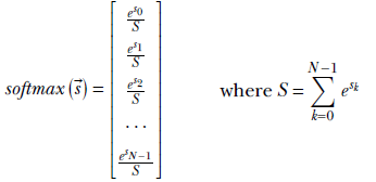
Equation 9.6
-
The vector has as many elements as possible classes.
-
The sum of the elements in the previous vector is 1.
-
The jth element of the vector represents the predicted probability of class j.
-
The formulation can handle arbitrary scores, including negative ones.
So in our example classification problem with the four classes (cat, dog, airplane, automobile), the score vector
![]() = [9.99 10 0.01 –10]
= [9.99 10 0.01 –10]
will yield the softmax vector
softmax (![]() ) = [0.497 0.502 2.30e–5 1.04e–9].
) = [0.497 0.502 2.30e–5 1.04e–9].
The probability of cat is 0.497, and the probability of dog is slightly higher, 0.502. The probabilities of airplane and automobile are much lower: the neural network predicts that the image is that of a dog, but it is not very confident; it could also be a cat.
Why the name softmax?
The softmax function is a smooth (differentiable) approximation to the argmaxonehot function, which emits a one-hot vector corresponding to the index of the max score. The argmaxonehot function is discontinuous. To see this, consider a pair of two class score vectors:
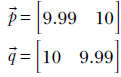
Performing an argmaxonehot operation on them will yield the following one-hot vectors, respectively:
Thus we see that the vectors argmaxonehot(![]() ) and argmaxonehot(
) and argmaxonehot(![]() ) are significantly far from each other, even though the points
) are significantly far from each other, even though the points ![]() and
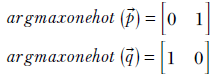
and ![]() are very close to each other. On the other hand, the corresponding softmax vectors are
are very close to each other. On the other hand, the corresponding softmax vectors are
Although the predicted classes still match those from the argmaxonehot vector, the softmax vectors are very close to each other. The closer the scores, the closer the softmax probabilities. In other words, the softmax is continuous.
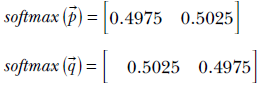
Figure 9.2 depicts this geometrically. The argmaxonehot functions as a function of the score vector [s0, s1] (for selecting classes 0 and 1, respectively) are shown in figures 9.2a and 9.2c. These are step functions on the (s0, s1) plane, with s0 = s1 being the decision boundary. Their softmax approximations are shown in figures 9.2b and 9.2d. In section 8.1, we introduced the 1D sigmoid function (see figure 8.1), which approximates the 1D step function. Here we see the higher-dimensional analog of that.
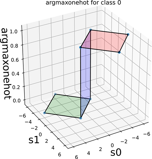
(a) Step function: z = 1 if s0 > = s1, else z = 0
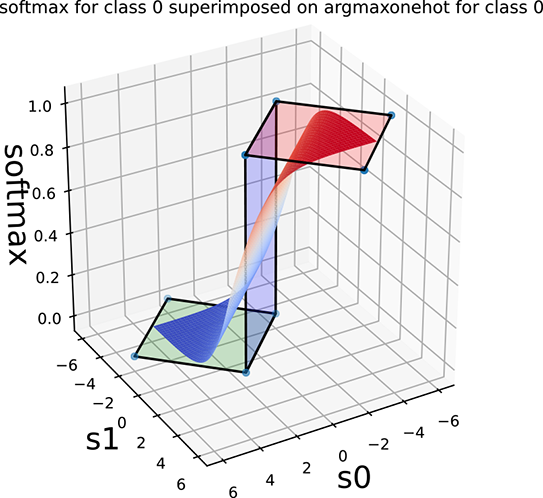
(b) Softmax: differential approximation of the step function
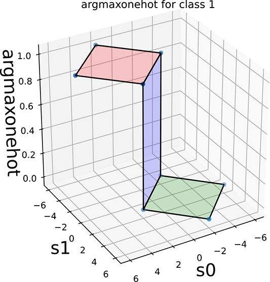
(c) Step function: z = 1 if s1 > = s0, else z = 0
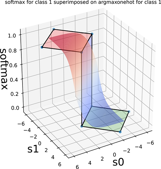
Figure 9.2 Two-class argmaxonehot and softmax (function of score vector [s0, s1]) on the (s0, s1) plane. The decision boundary is the 45o line s0 = s1.
Listing 9.4 PyTorch code for softmax
from torch.nn.functional import softmax      ①

scores = torch.tensor([9.99, 10, 0.01, -10]) ②

output = softmax(scores, dim=0)              ③
① Imports the softmax function
② Scores are typically raw, un-normalized outputs of a neural network.
③ Computes the softmax
9.1.6 Softmax cross-entropy loss
From the preceding discussion, it should be clear that it is desirable to make the last layer of a classifier neural network a softmax layer. Then, given an input, the network will emit probabilities for each class. During training, we can evaluate the loss on these probabilities with regard to the known GT probabilities. This can be done via the CE loss (see section 9.1.3). Thus the softmax is often followed by the CE loss during classifier training. Consequently, the combination (softmax CE loss) is available as a single operation in many deep learning packages, such as PyTorch. This is convenient because we do not need to call softmax and then CE loss. But the deeper reason for combining them is that the combination tends to be numerically better.
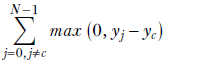
Let’s look at an example to see how the softmax CE loss changes as the output prediction changes. Consider the image classification problem again, where we’d like to classify whether an image contains one of four categories: cat (class 0), dog (class 1), airplane (class 2), or automobile (class 3). Figure 9.3 represents this visually. Suppose the image we’re classifying actually contains a dog class 1). The GT is represented as a one-hot vector [0 1 0 0]. If our classifier predicts the vector [0.498 0.502 0 0], it’s predicting both cat and dog with almost equal probability. This is a bad prediction because we would ideally expect it to confidently predict a dog (class 1). Consequently, the CE loss is high (0.688). On the other hand, if our classifier predicts [0.003 0.997 0 0], it is highly certain (with a probability of 0.997) that the image contains a dog. This is a good prediction, and hence the CE loss is low (0.0032). Softmax CE loss is probably the most popular loss method used for training in classifiers at the moment.
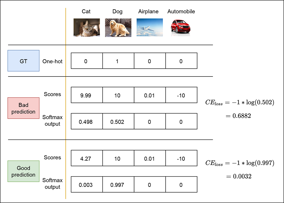
Figure 9.3 Softmax output and cross-entropy loss for good and bad output predictions
NOTE Fully functional code for softmax CE loss, executable via Jupyter Notebook, can be found at http://mng.bz/g1a8.
Listing 9.5 PyTorch code for softmax cross-entropy loss
from torch.nn.functional import cross_entropy

scores = torch.tensor([[9.99, 10, 0.01, -10]])

y_gt = torch.tensor([1])            ①

loss = cross_entropy(scores, y_gt)  ②
① Ground truth class index Ranges from 0 to _ –1
② Computes the softmax cross-entropy loss
9.1.7 Focal loss
As training progresses, where should we focus our attention? This question becomes especially significant when there is data imbalance, meaning the number of training data instances available for some classes is significantly smaller than others. In such cases, not all training data is equally important. We have to use our training data instances wisely.
Intuitively, the greater bang for the buck is trying to improve the training data instances that are not doing well. In other words, instead of trying to squeeze out every bit of juice from the examples in which the network is doing well (the so-called “easy” examples), it is better to focus on the examples where the network is not doing as well (“hard” examples).
To stop focusing on easy examples and focus instead on hard examples, we can put more weight on the loss from training data instances that are far from the GT, and vice versa: that is, put less weight on the loss from training data instances that are close to GT. Consider the binary CE loss of equation 9.4 one more time. The loss for the ith training instance can be rewritten as follows:
NOTE Going forward in this subsection, we drop the superscript (i) for the sake of notational simplification, although it remains implied.
Now, when the GT is class 1 (that is, ȳ = 1), the entity (1−y) measures the departure of the prediction from GT. We can multiply the loss by this to weigh down the losses from good predictions and weigh up the losses from bad predictions. In practice, we multiply by (1−y)γ for some value of γ (such as γ = 2). Similarly, when the GT is class 0 (that is, ȳ = 0), the entity y measures the departure of the prediction from the GT. In this case, we multiply the loss by yγ. The overall loss then becomes
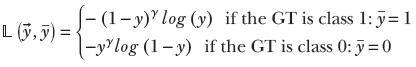
We can have a somewhat simplified expression
![]()
Equation 9.7
where
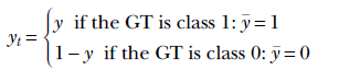
Equation 9.7 is the popular expression of focal loss. Its graph at various values of γ is shown in figure 9.4. Note how the loss becomes more and more subdued as the probability of the GT increases toward the right until it flattens out at the bottom.
NOTE Fully functional code for focal loss, executable via Jupyter Notebook, can be found at http://mng.bz/g1a8.
Listing 9.6 PyTorch code for focal loss
def focal_loss(y, y_gt, gamma):
    y_t = (y_gt * y) + ((1 - y_gt) * (1 - y)) ①

    loss = -1 * torch.pow((1 - y_t), gamma) * torch.log(y_t)
    return loss
① yt = y if ygt is 1
yt = 1 − y if ygt is 0
9.1.8 Hinge loss
The softmax CE loss becomes zero only under the ideal condition: the correct class has a finite score, and other classes have a score of negative infinity. Hence, that loss will continue to push the network toward improvement until the ideal is achieved (which never happens in practice). Sometimes we prefer to stop changing the network when the correct class has the maximum score, and we do not care about increasing the distance between correct and incorrect scores any further. This is where hinge loss comes in.
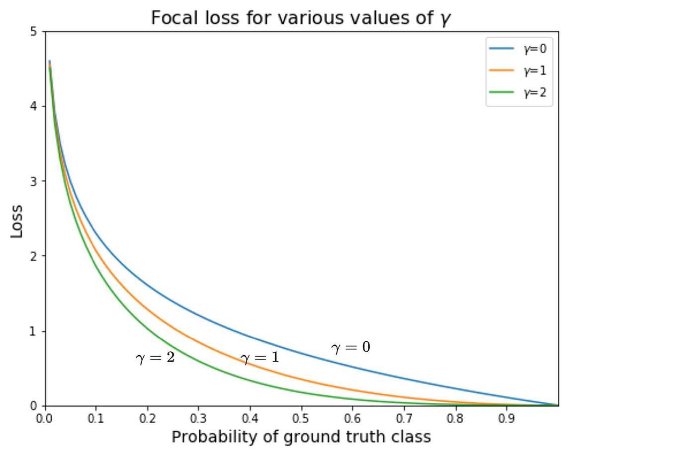
Figure 9.4 Focal loss graph (various γ values)
A hinged door opens in one direction but not in the other direction. Similarly, a hinge loss function increases if a certain goodness criterion is not satisfied but becomes zero (and does not reduce any further) if the criterion is satisfied. This is akin to saying, “If you are not my friend, the distance between us can vary from small to large (unboundedly), but I don’t distinguish between friends. All my friends are at a distance of zero from me.”
Multiclass support vector machine loss: Hinge loss for classification
Consider again our old friend, the classifier that predicts whether an image contains a cat (class 0), dog class 1), airplane (class 2), or automobile (class 3). Our classifier emits an output vector ![]() corresponding to an input image. Here, the outputs are scores: yj is the score corresponding to the jth class. (In this subsection, we have dropped the superscripts indicating the training data index to simplify notations.)
corresponding to an input image. Here, the outputs are scores: yj is the score corresponding to the jth class. (In this subsection, we have dropped the superscripts indicating the training data index to simplify notations.)
Given a (training data instance, GT label) pair (![]() , c) (that is, the GT class corresponding to the input
, c) (that is, the GT class corresponding to the input ![]() is c), the multiclass support vector machine (SVM) loss is
is c), the multiclass support vector machine (SVM) loss is
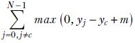
Equation 9.8
where m is a margin usually m = 1).
To understand this, consider the equation without the margin first:
In equation 9.8, we are summing over all the classes except the one that matches the GT. In other words, we are summing over only the incorrect classes. For these, we want the score yj to be smaller than the score yc for the correct class. There are two possibilities:
-
Good output—Incorrect class score less than correct class score:
yj − yc < 0 ⟹ max(0, yj − yc) = 0
The contribution to the loss is zero (we do not distinguish between correct scores: all friends are at zero distance). -
Bad output—Incorrect class score more than correct class score:
yj > yc ⟹ max(0, yj – yc) = yj − yc
The contribution to the loss is positive (non-friends are at a positive distance that varies with the degree of non-friendness).
In practical settings, the margin is set to a positive number usually 1) to penalize predictions where the score of the correct class is marginally greater than that of the incorrect classes. This forces the classifier to learn to predict the correct class with high confidence. Figure 9.8 shows how hinge loss differs for good and bad output predictions.
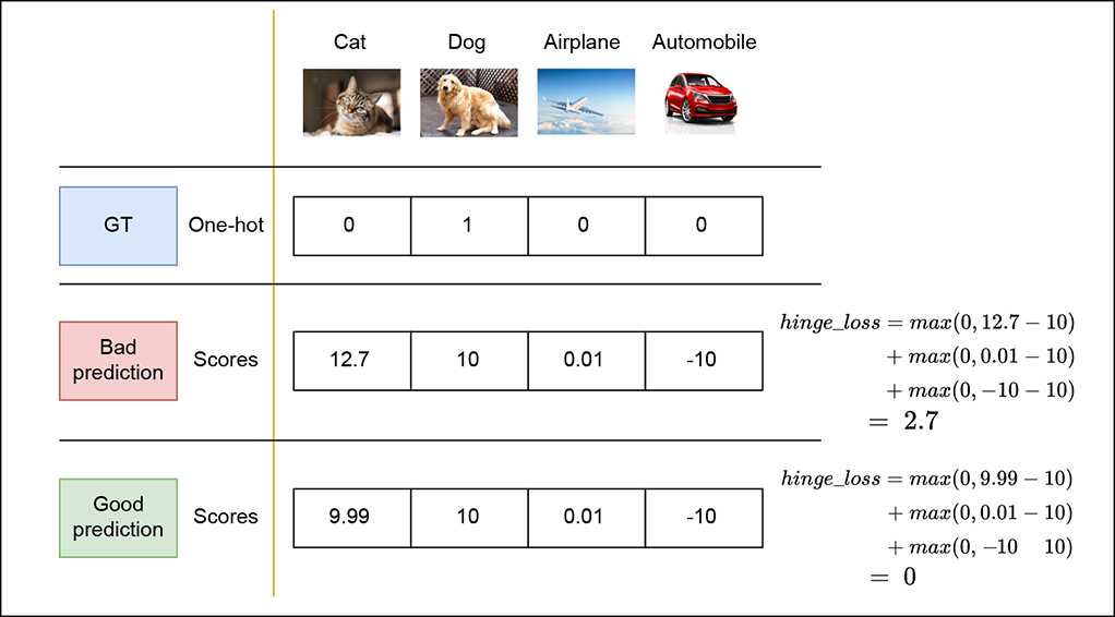
Figure 9.5 Hinge loss for good and bad output predictions
One mental model to have about the multiclass SVM loss is that it is lazy. It stops changing as soon as the correct class score exceeds the incorrect scores by the margin m. The loss does not change if the correct class score goes still higher, which means it does not push the machine to improve beyond that point. This behavior is different from the softmax CE loss, which tries to push the machine to achieve an infinite score for the correct class.
9.2 Optimization
Neural network models define a loss function that estimates the badness of the network’s output. During supervised training, the output on a particular training instance input is compared to a known output GT) for that particular training instance. The difference between the GT and the network-generated output is called loss. We can sum up the losses from individual training data instances and compute the total loss over all the training data.
These losses are, of course, functions of the network parameters, ![]() ,
, ![]() . We can imagine a space whose dimensionality is dim(
. We can imagine a space whose dimensionality is dim(![]() ) + dim(
) + dim(![]() ). At each point in this space, we have a value for the total training loss. Thus, we can imagine a loss surface—a surface whose height represents the loss value—defined over the high-dimensional domain of network parameters (weights and biases).
). At each point in this space, we have a value for the total training loss. Thus, we can imagine a loss surface—a surface whose height represents the loss value—defined over the high-dimensional domain of network parameters (weights and biases).
Optimization is nothing but finding the lowest point on this surface. During training, we start with random values of network parameters: this is akin to starting at a random point on the surface. Then we constantly move locally downhill on the loss surface in the direction of the negative gradient. We hope this eventually takes us to the minimum or a sufficiently low point. Continuing our analogy of the loss surface as a ravine, the minimum is at sea level. This minimum provides us with the network parameter values (weights and biases) that will yield the least loss on the training data. If the training data set adequately represents the problem, the trained model will perform well on unseen data.
This process of traveling toward the minimum, the iterative updating of weights and biases to have minimal loss over the training dataset, is called optimization. The basic math was introduced in section 8.4.2 (equation 8.12). Here we study many practical nuances and variants.
At every iteration, we update the weights and biases, so if t denotes the iteration number, ![]() t denotes the weight values at iteration t, δ
t denotes the weight values at iteration t, δ![]() t denotes the weight updates at iteration t, and so on:
t denotes the weight updates at iteration t, and so on:
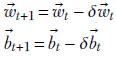
Equation 9.9
The basic update is along the direction of the negative gradient (see equation 8.12):
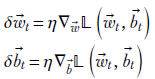
Equation 9.10
Here, 𝕃(![]() t,
t, ![]() t) denotes the loss at iteration t. Ideally, we should evaluate the loss on every training data instance and average them. But that would imply that we must process every training data instance for every iteration, which is prohibitively expensive. Instead, we use sampling see section 9.2.2):
t) denotes the loss at iteration t. Ideally, we should evaluate the loss on every training data instance and average them. But that would imply that we must process every training data instance for every iteration, which is prohibitively expensive. Instead, we use sampling see section 9.2.2):
-
The constant η is called the learning rate (LR). A larger LR results in bigger steps (bigger adjustments to weights and biases per update) and vice versa. We use larger values of LR in the beginning: when the network is completely untrained, we want to take large steps toward the minimum. When we are close to the minimum, on the other hand, we want to take smaller steps, lest we overshoot it. The LR is typically a small number, like η = 0.01.
-
In stochastic gradient descent (SGD; a popular approach), the LR η is typically held constant during an epoch (an epoch is a single pass over all the training data). Then the LR is decreased after one or more epochs. This process is called learning rate decay. So, the LR is not exactly a constant. We could have written it ηt to indicate the temporal nature, but we chose to keep it simple because (in SGD, at least) it changes infrequently.
We have to reevaluate the loss and its gradients in each iteration since their values will change in every iteration, because the weights and biases of the underlying neural network are changing.
How many iterations are necessary? Typically, this is a large number. We iterate multiple times over the entire training dataset. A typical training session has multiple epochs. In this context, note that for proper convergence, it is extremely important to randomly shuffle the order of occurrence of the training data after every epoch. In the following sections, we look at some practical nuances of the process.
9.2.1 Geometrical view of optimization
This topic is described in detail in section 8.4.2. You are encouraged to revisit that discussion if necessary.
Overall, neural network optimization is an iterative process. Ideally, in each iteration, we compute the gradient of the loss with respect to the current parameters (weights and biases) and obtain improved values for them by moving in the direction of the negative gradient.
9.2.2 Stochastic gradient descent and minibatches
How do we compute the gradient of the loss function? The loss is different for every training data instance. The sensible thing to do is to average them out. But as we mentioned earlier, that leads to a practical problem: we would have to process the entire training dataset on every iteration. If the size of the training dataset is n, an epoch is an O(n2) operation every iteration, we have to process all of the n training data instances to compute the gradient, and an epoch has n iterations). Since n is a large number, often in the millions, O(n2) is prohibitively expensive.
In SGD, we do not average over the entire training data set to produce the gradient. Instead, we average over a random sampled subset of the training data. This randomly sampled subset of training data is called a minibatch. The gradient is computed by averaging the loss over the minibatch (as opposed to the entire training dataset). This gradient is used to update the weight and bias parameters.
9.2.3 PyTorch code for SGD
Now, let’s implement SGD in PyTorch.
NOTE Fully functional code for SGD, executable via Jupyter Notebook, can be found at http://mng.bz/ePyG.
Let’s consider the example discussed in section 6.9. Our goal is to build a model that can predict whether a Statsville resident is a man, woman, or child using height and weight as input data. For this purpose, let’s assume we have a large dataset X containing the heights and weights of various Statsville residents. X is of shape (num_samples,2), where each row represents the (height, weight) pair of a single resident. The corresponding labels are stored in ygt, which contains num_samples elements. Each row of ygt can be 0, 1, or 2, depending on whether the resident is a man, woman, or child. Figure 9.6 shows an example distribution of X.
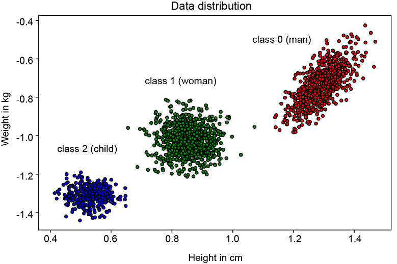
Figure 9.6 Height and weight of various Statsville residents. Class 0 (man) is represented by the right-most cluster, class 1 (woman) by the middle cluster, and class 2 (child) by the left-most cluster.
Before training a model, we must first convert the data into a training-friendly format. We subclass torch.utils.data.Dataset to do so and implement the __len__ and __getitem__ methods. The ith training data instance can be accessed by calling data_set[i]. Remember that in SGD, we feed in minibatches that contain batch_size elements in every iteration. This can be achieved by calling the __getitem__ method batch_size times. However, instead of doing this ourselves, we use PyTorch’s DataLoader, which gives us a convenient wrapper. Using DataLoader is recommended in production settings because it provides a simple API through which we can (1) create minibatches, 2) speed up data-loading times via multiprocessing, and (3) randomly shuffle data in every epoch to prevent overfitting. The following code creates a custom PyTorch data set.
Listing 9.7 PyTorch code to create a custom dataset
from torch.utils.data import Dataset, DataLoader

class StatsvilleDataset(Dataset):                ①
    def __init__(self, X, y_gt):
        self.X = X
        self.y_gt = y_gt

    def __len__(self):                           ②
        return len(self.X)

    def __getitem__(self, i):                    ③
        return self.X[i], self.y_gt[i]

dataset = StatsvilleDataset(X, y_gt)             ④

data_loader = DataLoader(dataset, batch_size=10, ⑤
                       shuffle=True)
① Subclasses torch.utils.data.Dataset
② Returns the size of the data set
③ Returns the ith training data element
④ Instantiates the data set
⑤ Instantiates the data loader with a batch size of 10 and shuffle on
Our next step is to create a classifier model that can take the height and weight data (X) as input and predict the output class. Here, we create a simple neural network model that consists of two linear layers followed by a softmax layer. The output of the softmax layer has three values representing the probability of each of the three classes (man, woman, and child), respectively. Note that in the forward pass, we don’t call the softmax layer because our loss function, PyTorch’s CE loss, expects raw, un-normalized scores as input. Hence we pass the output of the second linear layer to the loss function. However, during prediction, we pass the scores to the softmax layer to get a probability vector and then take an argmax to get the predicted class. Notice that we have a function to initialize the weights of the linear layers: this is important because the starting value of the weights can often affect convergence. If the model starts too far from the minimum, it may never converge.
Listing 9.8 PyTorch code to create a custom neural network model
class Model(torch.nn.Module):                                     ①
    def __init__(self, input_size, hidden_size, output_size):
        super(Model, self).__init__()
        self.linear1 = torch.nn.Linear(input_size, hidden_size)   ②
        self.linear2 = torch.nn.Linear(hidden_size, output_size)
        self.softmax = torch.nn.Softmax(dim=1)

    def forward(self, X):                                         ③
        scores = self.linear2(self.linear1(X))
        return scores

    def predict(self, X):                                         ④
        scores = self.forward(X)
        y_pred = torch.argmax(self.softmax(scores), dim=1)
        return y_pred


def initialize_weights(m):
    if isinstance(m, torch.nn.Linear):
        torch.nn.init.xavier_uniform_(m.weight.data)              ⑤
        torch.nn.init.constant_(m.bias.data, 0)

model = Model(input_size=2, hidden_size=100, output_size=3)
model.apply(initialize_weights)
① Subclasses torch.nn.Module
② Instantiates the linear layers and the softmax layer
③ Feeds forward the input through the two linear layers
④ Predicts the output class index
⑤ Initializes the weights to help the model converge better
Now that we have our data set and model, let’s define our loss function and instantiate our SGD optimizer.
Listing 9.9 PyTorch code for a loss function and SGD optimizer
loss_fn = torch.nn.CrossEntropyLoss()
optimizer = optim.SGD(model.parameters(), lr=0.02) ①
① Instantiates the SGD optimizer with learning rate = 0.02
Now we define the training loop, which is essentially one pass over the entire dataset. We iterate over the dataset in batches of size batch_size, run the forward pass, compute the gradients, and update the weights in the direction of the negative gradient. Note that we call optimizer.zero_grad() in every iteration to prevent the accumulation of gradients from the previous steps.
Listing 9.10 PyTorch code for one training loop
def train_loop(epoch, data_loader, model, loss_fn, optimizer):
    for X_batch, y_gt_batch in data_loader:                   ①

        scores = model(X_batch)                               ②

        loss = loss_fn(scores, y_gt_batch)                    ③

        optimizer.zero_grad()                                 ④

        loss.backward()                                       ⑤

        optimizer.step()                                      ⑥
① Iterates through the data set in batches
② Feeds forward the model to compute scores
③ Computes the cross-entropy loss
④ Clears the gradients accumulated from the previous step
⑤ Runs backpropagation and computes the gradients
⑥ Updates the weights
With this, we are ready to train our model. The following code shows how to do so. Figure 9.7 shows the output predictions and loss at the end of every epoch.
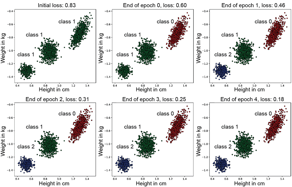
Figure 9.7 Model predictions at the end of every epoch. Notice how the loss is reduced with every epoch. In the beginning, all training data points are wrongly classified as class 1. After the end of epoch 1, most of the training data is classified correctly, and the distribution of the classifier’s output has become close to the ground truth. The loss continues to decrease until epoch 4 although the improvements are harder to see visually).
Listing 9.11 PyTorch code to run the training loop num_epochs times
num_epochs = 2
for epoch in range(num_epochs):
    train_loop(epoch, data_loader, model, loss_fn, optimizer)
9.2.4 Momentum
For real-life loss surfaces in high dimensions, the ravine analogy is quite appropriate. A loss surface is hardly like a porcelain cup with smooth walls; it is much more like the walls of the Grand Canyon (see figure 9.8). Furthermore, the gradient estimate (usually done over a minibatch) is noisy. Consequently, gradient estimates are never aligned in one direction—they tend to go hither and thither. Nonetheless, most of them tend to have a good downhill component. The other (non-downhill component) is somewhat random (see figure 9.8). So if we average them, the downhill components reinforce each other and are strengthened, while the non-downhill components cancel each other and are weakened.

Figure 9.8 Momentum. Noisy stochastic gradient estimates at different points on the loss surface (thick solid arrows) are not aligned in direction, but they all have a significant downhill component (thin solid arrows). The non-downhill components thin dashed arrows) point in random directions. Hence, averaging tends to strengthen the downhill component and cancel out the non-downhill components.
Furthermore, if there is a small flat region with downhill areas preceding and following it, the vanilla gradient-based approach will get stuck in the small flat region (since the gradient there is zero). But averaging with the past allows us to have nonzero updates that take the optimization out of the local small flat region so that it can continue downhill.
A good mental picture in this context is that of a ball rolling downhill. The surface of the hill is rough, and the ball is not going directly downward. Rather, it takes a zigzag path. But as it travels, it gathers downward momentum, and its downward velocity becomes greater.
Following this theory, we take the weighted average of the gradient computed at this iteration with the update used in the previous iteration:
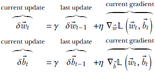
Equation 9.11
where γ, η are positive constants with values less than 1. The weights and bias parameters are updated in the usual fashion using equation 9.9.
Unrolling the recursion of the momentum equation
Unraveling the recursive equation 9.11, we see
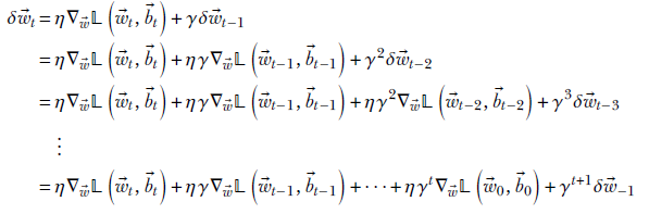
Assuming δ![]() −1 = 0, we get
−1 = 0, we get
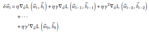
Equation 9.12
Thus,
-
We are taking a weighted sum of the gradients from past iterations. This is not quite a weighted average, though, as explained later.
-
Older gradients are weighted by higher powers of γ. Since γ < 1, weights decrease with age long-past iterations have less influence).
-
The sum of the weights of the gradients, going backward from now to the beginning of time (the 0th iteration), is
![]()
Now, using Taylor expansion,
Thus the sum of the weights of the past gradients in momentum-based gradient descent is η/(1–γ) ≠ 1. In other words, this is not quite a weighted average (where the weights should sum up to 1). This is a somewhat undesirable property and is rectified in the Adam algorithm discussed later.
A similar analysis can be done for the biases.
9.2.5 Geometric view: Constant loss contours, gradient descent, and momentum
Consider a network with a tiny two-element weight vector ![]() and no bias. Further, suppose that the loss function is 𝕃 = ||
and no bias. Further, suppose that the loss function is 𝕃 = ||![]() ||2 = w02 + w12. The constant loss contours are concentric circles with the origin as the center. The radius of the circle indicates the loss magnitude.
||2 = w02 + w12. The constant loss contours are concentric circles with the origin as the center. The radius of the circle indicates the loss magnitude.
If we move along the circle’s circumference, the loss does not change. The loss changes maximally along the orthogonal direction to that: the radius of the circle. This intuitive observation is confirmed by evaluating the gradient
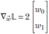
Thus the gradient is along the radius, and the negative gradient direction is radially inward. So the loss decreases most rapidly if we move radially inward. If we move orthogonal to the radius (that is, along the circumference), the loss remains unchanged; of course, we are moving along the constant loss contour.
Optimization then takes us from outer, larger-radius circles to inner, smaller-radius circles. The minimum is at the origin; ideally, optimization should stop once we reach the origin.
Figure 9.9 shows optimization for a simple loss function 𝕃 = ||![]() ||2 = w02 + w12. We start at an arbitrary pair of weight values and repeatedly update them via equation 9.9. For figure 9.9a, we use update without momentum (equation 9.10). For figure 9.9b, we use update with momentum (equation 9.11).
||2 = w02 + w12. We start at an arbitrary pair of weight values and repeatedly update them via equation 9.9. For figure 9.9a, we use update without momentum (equation 9.10). For figure 9.9b, we use update with momentum (equation 9.11).
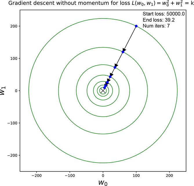
(a) A trajectory through constant loss contours for gradient descent without momentum
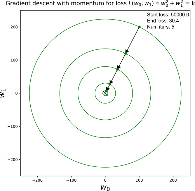
(b) A trajectory through constant loss contours for gradient descent with momentum
Figure 9.9 Constant loss contours and optimization trajectory for the loss function 𝕃 = ||![]() ||2 = w02 + w12. The loss surface is a cone with its apex on the origin and its base a circle in a plane parallel to the w0, w1 plane. Optimization takes us down the cone toward smaller and smaller cross-sections as we approach the minimum at the origin. Updates are shown with arrows. Note how the momentum version arrives at a smaller circle in fewer steps.
||2 = w02 + w12. The loss surface is a cone with its apex on the origin and its base a circle in a plane parallel to the w0, w1 plane. Optimization takes us down the cone toward smaller and smaller cross-sections as we approach the minimum at the origin. Updates are shown with arrows. Note how the momentum version arrives at a smaller circle in fewer steps.
When the constant loss contours are concentric circles with the origin as the center, the loss surface is a cone with its apex on the origin. The cross sections are circles on planes parallel to the w0, w1 plane. Optimization takes us down the inner walls of the cone through smaller and smaller circular cross-sections as we approach the minimum. The global minimum is at the origin and corresponds to zero loss. The zero-loss contour is a circle with a zero radius, which is effectively a single point: the origin.
In both cases, progress slows down (step sizes become smaller) as we approach the minimum. This is because the magnitude of the gradient becomes smaller and smaller as we get closer to the minimum (imagine a bowl: it becomes flatter as we get closer to the bottom). However, this effect is countered to a certain extent if we have momentum. So, we can see that we need fewer steps to reach a circle with a smaller radius when we have momentum.
9.2.6 Nesterov accelerated gradients
One problem with momentum-based gradient descent is that it may overshoot the minimum. This can be seen in figure 9.10a where the loss decreases through a series of updates and then, when we are close to the minimum, an update (shown with a dotted arrow) overshoots the minimum and increases the loss (shown with a dotted circle).
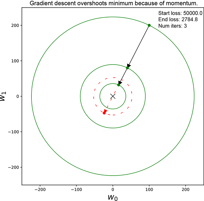
(a) Momentum gradient descent overshooting the minimum. Loss decreases for a while and then increases dotted circle and arrow)
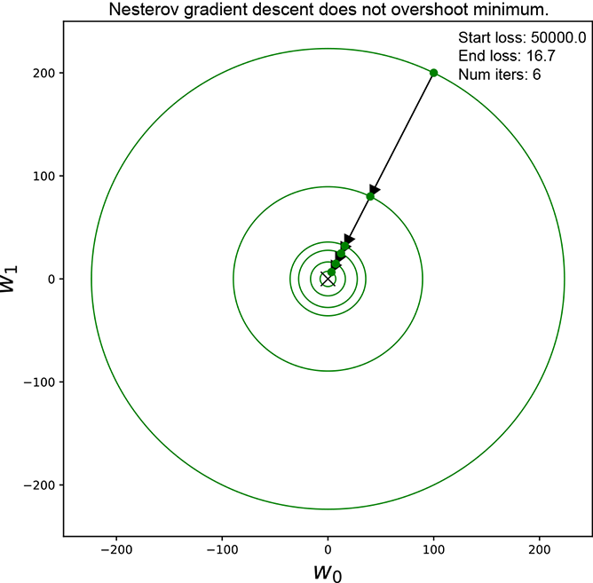
(b) Nesterov reduces the step size when we are about to overshoot the minimum.
Figure 9.10 Figure (a) shows momentum-based gradient descent overshooting the minimum. Over-shooting the update is shown with a dotted arrow. A circle with a radius larger than the last step is shown with a dotted outline. Nesterov does better by taking smaller steps when overshooting is imminent.
This is the phenomenon that Nesterov’s accelerated gradient-based optimization tries to tackle.
In Nesterov’s technique, we do the following:
-
Estimate where this update will take us (that is, the destination point) by adding the previous step’s update to the current point.
-
Compute the gradient at the estimated destination point. This is where the approach differs from the vanilla momentum-based approach, which takes the gradient at the current point.
-
Take a weighted average of the gradient (at the estimated destination point) with the previous step’s update. That is the update for the current step.
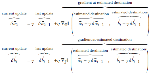
Equation 9.13
where γ, η are constants with values less than 1. The weights and biases are updated in the usual fashion using equation 9.9.
Why does this help? Well, consider the following:
-
When we are somewhat far away from the minimum (no possibility of overshooting), the gradient at the estimated destination is more or less the same as the gradient at the current point, so we progress toward the minimum in a fashion similar to momentum-based gradient descent.
-
But when we are close to the minimum and the current update may potentially take us past it (see the dotted arrow in figure 9.10a), the gradient at the estimated destination will lie on the other side of the minimum. As before, imagine this loss surface as a cone with its apex at the origin and base above the apex. We have traveled down one of the cone’s side walls and just started climbing back up. Thus the gradient at the estimated destination is in the opposite direction from the previous step. When we take their weighted average, they will cancel each other in some dimensions, resulting in a smaller magnitude. The resulting smaller step will mitigate the overshooting phenomenon.
NOTE Fully functional code for momentum and Nesterov accelerated gradients, executable via Jupyter notebook, can be found at http://mng.bz/p9KR.
9.2.7 AdaGrad
The momentum-based optimization approach (equation 9.11) and the Nesterov approach (equation 9.13) both suffer from a serious drawback: they treat all dimensions of the parameter vectors ![]() ,
, ![]() equally. But the loss surface is not symmetrical in all dimensions. The slope can be high along some dimensions and low along others. We cannot control everything with a single LR for all the dimensions. If we set the LR high, the high-slope dimensions will exhibit too much variance. If we set it low, the low-slope dimensions will barely progress toward the minimum.
equally. But the loss surface is not symmetrical in all dimensions. The slope can be high along some dimensions and low along others. We cannot control everything with a single LR for all the dimensions. If we set the LR high, the high-slope dimensions will exhibit too much variance. If we set it low, the low-slope dimensions will barely progress toward the minimum.
What we need is per-parameter LR. Then each LR will adapt to the slope of its particular dimension. This is what AdaGrad tries to achieve. Dimensions with historically larger gradients have smaller LRs, while dimensions with historically smaller gradients have larger LRs.
How do we keep track of the historic magnitudes of gradients? To do this, AdaGrad maintains a state vector in which it accumulates the sum of the squared partial derivatives for each dimension of the gradient vector seen so far during training:
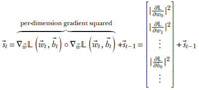
where ∘ denotes the Hadamard operator (elementwise multiplication of the two vectors). We can express the previous equation a bit more succinctly as
![]()
Unrolling the recursion, we get
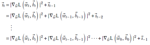
assuming ![]() −1 = 0,
−1 = 0, ![]() t is a vector that holds the cumulative sum over all training iterations of the squared slope for each dimension. For the dimensions with historically high slopes, the corresponding element of
t is a vector that holds the cumulative sum over all training iterations of the squared slope for each dimension. For the dimensions with historically high slopes, the corresponding element of ![]() t is large, and vice versa. The overall update vector looks like this:
t is large, and vice versa. The overall update vector looks like this:
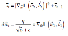
Equation 9.14
Here ϵ is a very small constant added to prevent division by zero. Then we use equation 9.9 to update the weights as usual. A parallel set of equations exist for the bias.
Using AdaGrad, in the loss gradient, the dimensions that have seen big slopes in earlier iterations are given less importance during the update. We emphasize the dimensions that have not seen much progress in the past. This is a bit like saying, “I will pay less attention to a person who speaks all the time, and I will pay more attention to someone who speaks infrequently.”
9.2.8 Root-mean-squared propagation
A significant drawback of the AdaGrad algorithm is that the magnitude of the vector ![]() t keeps increasing as iteration progresses. This causes the LR for all dimensions to become smaller and smaller. Eventually, when the number of iterations is high, the LR becomes close to zero, and the updates do hardly anything; progress toward the minimum slows to a virtual halt. Thus AdaGrad is an impractical algorithm to use in real life, although the idea of per-component LR is good.
t keeps increasing as iteration progresses. This causes the LR for all dimensions to become smaller and smaller. Eventually, when the number of iterations is high, the LR becomes close to zero, and the updates do hardly anything; progress toward the minimum slows to a virtual halt. Thus AdaGrad is an impractical algorithm to use in real life, although the idea of per-component LR is good.
Root mean squared propagation (RMSProp) addresses this drawback without sacrificing the dimension-adaptive nature of AdaGrad. Here again there is a state vector, but its equation is
![]()
Compare this with the state vector equation in AdaGrad:
![]()
They are almost the same, but the terms are weighted by (1−γ) and γ, where 0 < γ < 1 is a constant. This particular pair of weights in a recursive equation has a very interesting effect. To see it, we have to unroll the recursion:
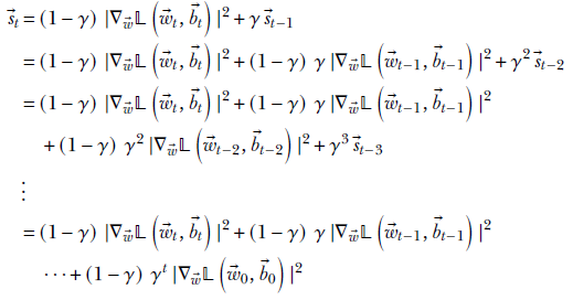
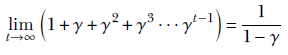
Thus ![]() t is a weighted sum of the past term-wise squared gradient magnitude vectors. Going back from now to the beginning of time (the 0th iteration), the weights are (1−γ), (1−γ) γ, (1−γ) γ2, ⋯, (1−γ) γt. If we add these weights, we get
t is a weighted sum of the past term-wise squared gradient magnitude vectors. Going back from now to the beginning of time (the 0th iteration), the weights are (1−γ), (1−γ) γ, (1−γ) γ2, ⋯, (1−γ) γt. If we add these weights, we get
![]()
As the number of iterations becomes high (t → ∞), this becomes

where Taylor expansion has been used to evaluate the term in parentheses.
For a large number of iterations, the sum of the weights approaches 1. This implies that after many iterations, the RMSProp state vector effectively takes the weighted average of the past term-wise squared gradient magnitude vectors. With more iterations, the weights are redistributed and older terms become de-emphasized, but the overall magnitude does not increase. This eliminates the vanishing LR problem from AdaGrad. RMSProp continues de-emphasizing the dimensions with high cumulative partial derivatives with lower LRs, but it does so without making the LR vanishingly small.
The overall RMSProp update equations are
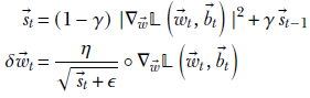
Equation 9.15
There is a parallel set of equations for the bias. The weights and bias parameters are updated in the usual fashion using equation 9.9.
9.2.9 Adam optimizer
Momentum-based gradient descent amplifies the downhill component more and more as iterations progress. On the other hand, RMSProp reduces the LR for dimensions that are seeing large gradients and vice versa to balance the progress rate along all dimensions.
Both of these are desirable properties. We want an optimization algorithm that combines them, and that algorithm is Adam. It is increasingly becoming the optimizer of choice for most deep learning researchers.
The Adam optimization algorithm maintains two state vectors:
![]()
Equation 9.16
![]()
Equation 9.17
where 0 < β1 < 1 and 0 < β2 < 1 are constants. Note the following:
-
Equation 9.16 is essentially the momentum equation of equation 9.11 with one significant difference. We have changed the term weights to β1 and (1−β1). As we’ve seen, with t → ∞, this results in the state vector being a weighted average of all the past gradients. This is an improvement over the original momentum scheme.
-
The second state vector is basically the one from the RMSProp equation 9.15.
Using these two state vectors, Adam creates the update vector as follows:
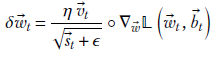
Equation 9.18
The ![]() t in the numerator pulls in the benefits of the momentum approach (with the enhancement of averaging). Otherwise, the equation is almost identical to the RMSProp; those benefits are also pulled in.
t in the numerator pulls in the benefits of the momentum approach (with the enhancement of averaging). Otherwise, the equation is almost identical to the RMSProp; those benefits are also pulled in.
Finally, the weights and bias parameters are updated in the usual fashion using equation 9.9.
Bias correction
The sum of weights of past values in the state vectors ![]() t,
t, ![]() t will approach ∞ only at large values of t. To improve the approximation at smaller values of t, Adam introduces a bias correction:
t will approach ∞ only at large values of t. To improve the approximation at smaller values of t, Adam introduces a bias correction:
![]()
Equation 9.19
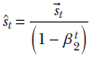
Equation 9.20
Instead of ![]() t and
t and ![]() t, we use the bias-corrected entities v̂t and ŝt in equation 9.18.
t, we use the bias-corrected entities v̂t and ŝt in equation 9.18.
Listing 9.12 PyTorch code for various optimizers
from torch import optim

sgd_optimizer = optim.SGD([params], lr=0.01)                   ①

sgd_momentum_optimizer = optim.SGD([params], lr=0.01,
                                    momentum=0.9)              ②

sgd_nesterov_momentum_optimizer = optim.SGD([params], lr=0.01, ③
                                    momentum=0.9, nesterov=True)

adagrad_optimizer = optim.Adagrad([params], lr=0.001)

rms_prop_optimizer = RMSprop([params], lr=1e-2,                ④
                       alpha=0.99)

adam_optimizer = optim.Adam([params], lr=0.001,
                       betas=(0.9, 0.999))
① Sets the learning rate to 0.01
② Sets the momentum to 0.9
③ Sets the Nesterov flag to True
④ Sets the smoothing constant to 0.99 (γ in 9.15)
9.3 Regularization
Suppose we are teaching a baby to recognize cars. We show them red cars, blue cars, black cars, large cars, small cars, medium cars, cars with round tops, cars with rectangular tops, and so on. Soon the baby’s brain realizes that there are too many varieties to remember them all by rote. So the brain starts forming abstractions: mysterious common features that occur together are stored in the baby’s brain with the label car. The brain has learned to classify an abstract entity called a car. Even though it fails to remember every car it has seen, it can recognize cars. We can say it has developed experience. And so it is with neural networks. We do not want our network to remember every training instance. Rather, we want the network to form abstractions that will enable it to recognize an object during inferencing even though the exact likeness of the object instance encountered during inferencing was never seen during training.
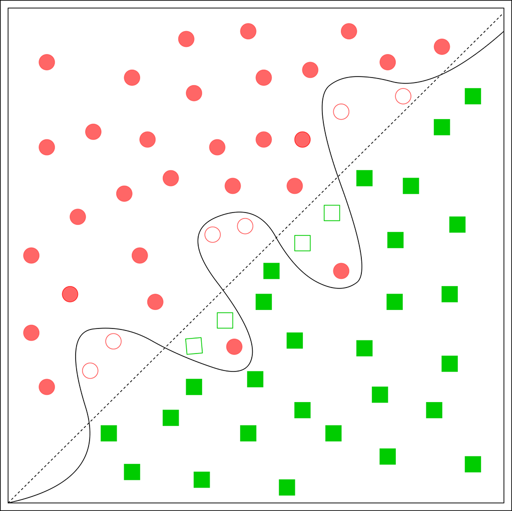
Figure 9.11 Overfitting: data points for a binary classifier. Points belonging to different classes are visually demarcated as squares and circles. Filled squares/circles indicate training data, and unfilled squares/circles indicate test data. There are some anomalous training data instances (filled circles in the square zone). The estimated decision boundary (solid line) has become wriggly to accommodate them, which is causing many test points (unfilled squares/circles) to be misclassified. The wiggly solid curve is an example of an overfitted decision boundary. If we had chosen a “simpler” decision boundary (dashed straight line), the two anomalous training points would have been misclassified, but the machine would have performed much better in tests.
9.3.1 Minimum descriptor length: An Occam’s razor view of optimization
Is the set of weights and biases that minimizes a particular loss function unique? Let’s examine a single perceptron (equation 7.3) with the output ϕ(![]() T
T![]() + b). Let’s say ϕ is the Heaviside step function (see section 7.3.1). Let
+ b). Let’s say ϕ is the Heaviside step function (see section 7.3.1). Let ![]() *, b* be the weights and biases minimizing the loss function. It is easy to see that the perceptron output remains the same if we scale the weights, like α
*, b* be the weights and biases minimizing the loss function. It is easy to see that the perceptron output remains the same if we scale the weights, like α![]() * for all positive real values of α. Thus the weight vector 7
* for all positive real values of α. Thus the weight vector 7![]() * will also minimize the loss function.
* will also minimize the loss function.
This is true in general for arbitrary neural networks (composed of many perceptrons): the set of weights and biases minimizing a loss function is non-unique. How does the neural network choose one? Which of them is correct? We can use the principle of Occam’s razor to answer that.
Occam’s razor is a philosophical principle. Its literal translation from Latin states, “Entities should not be multiplied beyond necessity.” This is roughly taken to mean among adequate explanations, the simplest one is the best. In machine learning, this principle is typically interpreted as follows:
Among the set of candidate neural network parameter values (weights and biases) that minimize the loss, the “simplest” one should be chosen.
The general idea is as follows. Suppose we are trying to minimize 𝕃(θ) (here we have used θ to denote ![]() and
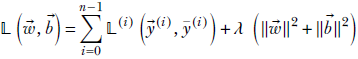
and ![]() together). We also want the solution to be as simple as possible. To achieve that, we add a penalty for departing from “simplicity” to the original loss term. Thus we minimize
together). We also want the solution to be as simple as possible. To achieve that, we add a penalty for departing from “simplicity” to the original loss term. Thus we minimize
𝕃(θ) + λR(θ)
Here,
-
The expression R(θ) indicates a measure for un-simplicity. It is sometimes called the regularization penalty. Adding a regularization penalty to the loss incentivizes the network to try to minimize un-simplicity R(θ) (or, equivalently, maximize simplicity) while trying to minimize the original loss term 𝕃(θ).
-
λ is a hyperparameter. Its value should be carefully chosen via trial and error. If λ is too low, this is akin to no regularization, and the network becomes prone to overfitting. If λ is too high, the regularization penalty will dominate, and the network will not adequately minimize the actual loss term.
There are two popular ways of estimating R(θ), outlined in sections 9.3.2 and 9.3.3, respectively. Both try to minimize some norm (length) of the parameter vector (which is basically a network descriptor). This is why regularization can be viewed as minimizing the descriptor length.
9.3.2 L2 regularization
In L2 regularization, we posit that shorter-length vectors are simpler. In other words, simplicity is inversely proportional to the square of the L2 norm (aka Euclidean norm). Thus,
R(θ) = (||![]() ||2+||
||2+||![]() ||2)
||2)
Overall, we minimize
Equation 9.21
Compare this with equation 9.2.
L2 regularization is by far the most popular form of regularization. From this point on, we often use 𝕃(![]() ,
, ![]() ) to mean the L2-regularized version (that is, equation 9.21). The hyperparameter λ is often called weight decay in PyTorch. Weight decay is usually set to a small number so that the second term of equation 9.21 the norm of the weight vector) does not drown the actual loss term. The following code shows how to instantiate an optimizer with regularization enabled.
) to mean the L2-regularized version (that is, equation 9.21). The hyperparameter λ is often called weight decay in PyTorch. Weight decay is usually set to a small number so that the second term of equation 9.21 the norm of the weight vector) does not drown the actual loss term. The following code shows how to instantiate an optimizer with regularization enabled.
Listing 9.13 PyTorch code to enable L2 regularization
from torch import optim

optimizer = optim.SGD([params], lr=0.2, weight_decay=0.01) ①
① Sets the weight decay to 0.01
(a) L1 regularization
(b) L2 regularization
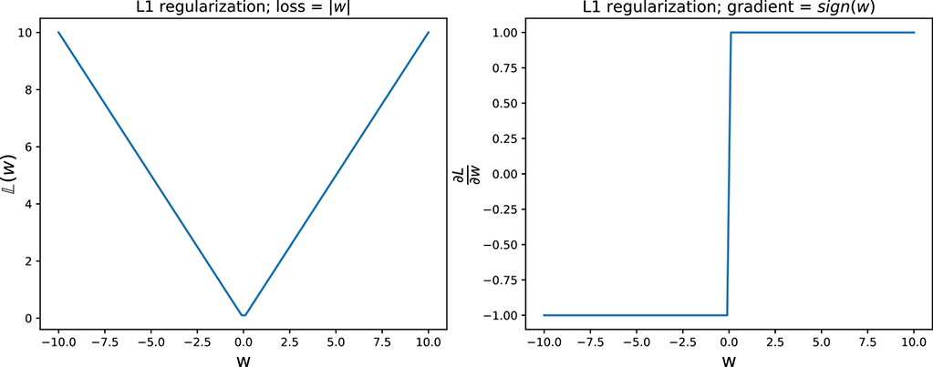
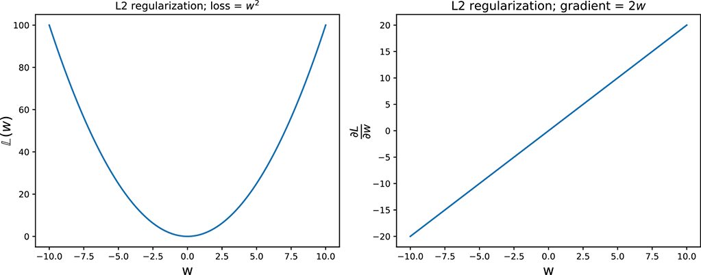
Figure 9.12 L1 and L2 regularization
9.3.3 L1 regularization
L1 regularization is similar in principle to L2 regularization, but it defines simplicity as the sum of the absolute values of the weights and biases:
R(θ) = (|![]() |+|
|+|![]() |)
|)
Thus, here we minimize
Equation 9.22
9.3.4 Sparsity: L1 vs. L2 regularization
L1 regularization tends to create sparse models where many of the weights are 0. In comparison, L2 regularization tends to create models with low (but nonzero) weights.
To understand this, consider figure 9.12, which plots the loss function and its derivative for both L1 and L2 regularization. Let w be a single element of the weight vector ![]() . In L1 regularization,
. In L1 regularization,
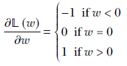
Since the gradient is constant for all values of w, L1 regularization pushes the weight toward 0 with the same step size at all values of w. In particular, the step toward 0 does not reduce in magnitude when close to 0. In L2 regularization,
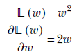
Here, the gradient keeps decreasing in magnitude as w approaches 0. Hence, w comes closer to 0 but may never reach 0 since the updates take smaller and smaller steps as w approaches 0. Therefore, L2 regularization produces more dense weight vectors than L1 regularization, which produces sparse weight vectors with many 0s.
9.3.5 Bayes’ theorem and the stochastic view of optimization
In sections 6.6.2 and 6.6.3, we discussed maximum likelihood estimation (MLE) and maximum a posteriori (MAP) in the context of unsupervised learning (you are encouraged to revisit those sections if necessary). Here, we study them in the context of supervised learning.
In the supervised optimization process, we have samples of the input and known output pairs (in the form of training data) ⟨![]() (i), ȳ(i)⟩. Of course, we can do the forward pass and generate the network output at each training data point
(i), ȳ(i)⟩. Of course, we can do the forward pass and generate the network output at each training data point
![]()
where θ is the network’s parameter set (representing weights and biases together).
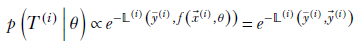
Suppose we view the sample training data generation as a stochastic process. We can model the probability of a training instance T(i) = ⟨ȳ(i), ![]() (i)⟩ given the current network parameters θ as
(i)⟩ given the current network parameters θ as
![]()
This makes intuitive sense. At an optimal value of θ, the network output f(![]() (i), θ) would match the GT ȳ(i). We want our model distribution to have the highest probability density at the location where the network output matches the GT. The probability density should fall off with distance from that location.
(i), θ) would match the GT ȳ(i). We want our model distribution to have the highest probability density at the location where the network output matches the GT. The probability density should fall off with distance from that location.
A little thought reveals that this Gaussian-like formulation, which leads to a regression-loss-like numerator, is not the only one possible. We can use any loss function in the numerator since all of them have the property of being minimum when the network output matches the GT and gradually increase as the mismatch grows. In general,
Assuming the training instances are mutually independent, the probability of the entire training dataset occurring jointly is the product of individual instance probabilities. If we denote the entire training dataset as T,
![]()
Then
At this point, we can take one of two possible approaches described in the next two subsections.
MLE-based optimization
In this approach, we choose the optimal value for the parameter set θ by maximizing the likelihood
![]()
This is equivalent to saying we will choose the optimal parameters θ such that the probability of occurrence of the training data is maximized. Thus the optimal parameter set θ* is yielded by
![]()
Obviously, the optimal θ that maximizes the likelihood is the one that minimizes 𝕃(θ). So, the maximum likelihood formulation is nothing but minimizing the total mismatch between predicted and GT output over the entire training dataset.
MAP optimization
By Bayes’ theorem (equation 6.1),
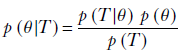
To estimate the optimal θ, we can also maximize the posterior probability on the left side of this equation. This is equivalent to saying we will choose the optimal parameters θ such that θ has the maximal conditional probability given the training dataset. Thus the optimal value for the parameter set θ is yielded by
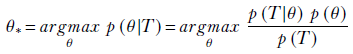
where the last equality is derived via Bayes’ theorem.
Observing the previous equation, we see that the denominator p(T) in the rightmost term does not involve θ and hence can be dropped from the optimization. So,
![]()
How do we model the a priori probability p(θ)? We can use Occam’s razor and say that we assign a higher a priori probability to smaller parameter values. Thus, we can say
![]()
Then the overall posterior probability maximization becomes
![]()
NOTE Maximizing this posterior probability is equivalent to minimizing the regularized loss. Maximizing the likelihood is equivalent to minimizing the un-regularized loss.
9.3.6 Dropout
In the introduction for section 9.3, we saw that too much expressive power (too many perceptron nodes) sometimes prevents the machine from developing general abstractions (aka experience). Instead, the machine may remember the training data instances (see figure 9.11). This phenomenon is called overfitting. We have already seen that one way to mitigate this problem is to add a regularization penalty—such as adding the L2 norm of the weights—to the loss to discourage the network from learning large weight values.
Dropout is another method of regularization. Here, somewhat crazily, we turn off random perceptrons in the network (set their value to 0) during training. To be precise, we attach a probability pil with the ith node (perceptron) in layer l. In any training iteration, the node (perceptron) is off with a probability of (1−p). Typically, dropout is only enabled during training and is turned off during inferencing.
What good does it do? Well,
-
Dropout prevents the network from relying too much on a small number of nodes. Instead, the network is forced to use all the nodes.
-
Equivalently, dropout encourages the training process to spread the weights to multiple nodes instead of putting much weight on a few nodes. This makes the effect somewhat similar to L2 regularization.
-
Dropout mitigates co-adaptation: a behavior whereby a group of nodes in the network behave in a highly correlated fashion, emitting similar outputs most of the time. This means the network could retain only one of them with no significant loss of accuracy.
Dropout simulates an ensemble of subnetworks
Consider a small three-node intermediate layer of some neural network with dropout. The kth input to this layer can turn on with probability pk. This means the probability of that input node turning off is (1−pk). We can express this with a binary stochastic variable δk for k = 0 or k = 1 or k = 2. This variable δk takes one of two possible values: 0 or 1. The probability of it taking the value 1 is pk. In other words, p(δk = 1) = pk, and p(δk = 0) = 1 − pk. The output of this small three-node layer with dropout can be expressed as
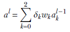
We have three variables δ0, δ1, and δ2, each of which can take two values. Altogether we have 23 = 8 possible combinations. Each combination leads to a subnode shown in figure 9.13. Each of these combinations has a probability of occurrence Pi, also shown in the figure. These observations lead to a very important insight:
The expected value of the output—that is, 𝔼(al)—is the same as the expected value of the output if we deployed the subnetworks in figure 9.13 randomly, with probabilities Pi.
Why does this matter? Well, given a problem, none of us know the right number of perceptrons for the network to deploy. One thing to do under these circumstances is to deploy networks of various strengths randomly and take an average of their outputs. We have just established that dropout (turning inputs off randomly) achieves the same thing. But deploying a network where inputs get turned on or off randomly is much simpler than deploying a large number of subnetworks. All we have to do is deploy a dropout layer.
PyTorch code for dropout
In section 9.2.3, we created a simple two-layer neural network classifier to predict whether a Statsville resident is a man, woman, or child based on height and weight data. In this section, we show the same model with dropout layers added. Note that dropout should be enabled only during training, not during inferencing. To do this in PyTorch, you can call model.eval() before running inferencing. This way, your training and inferencing code remains the same, but PyTorch knows under the hood when to include the dropout layers and when not to.
Listing 9.14 Dropout
class ModelWithDropout(torch.nn.Module):
    def __init__(self, input_size, hidden_size, output_size):
        super(Model, self).__init__()
        self.net = torch.nn.Sequential(
            torch.nn.Linear(input_size, hidden_size),
            torch.nn.Dropout(p=0.2),                 ①


            torch.nn.Linear(hidden_size, output_size),
            torch.nn.Dropout(p=0.2)
        )

    def forward(self, X):
        return self.net(X)
① Instantiates a dropout layer with a probability of dropout = 0.2
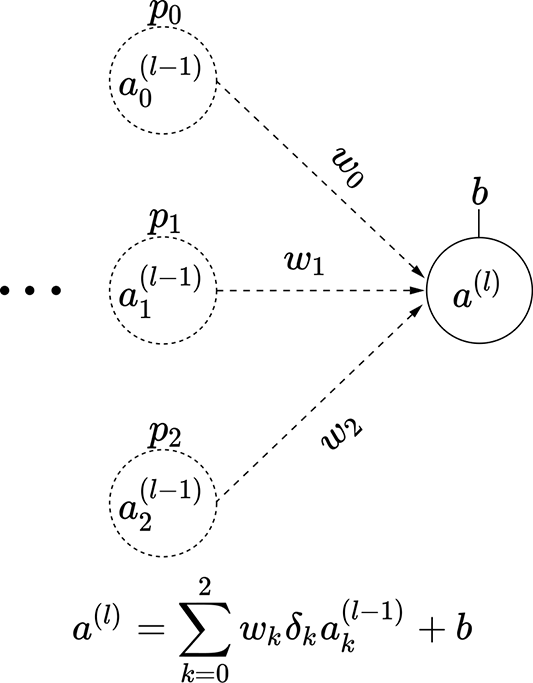
(a) Subnetwork 0: probability P0 = (1−p0) (1−p1) (1−p2)
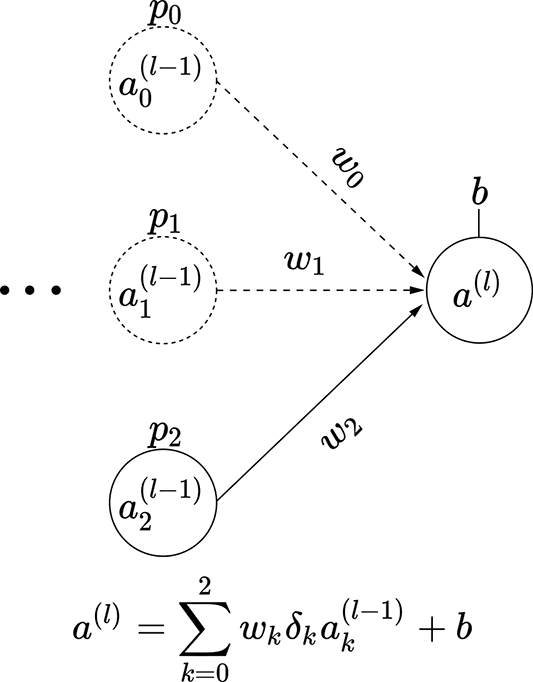
(b) Subnetwork 1: probability P1 = (1−p0) (1−p1) p2
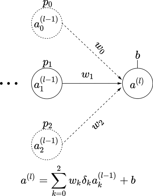
(c) Subnetwork 2: probability P2 = (1−p0 )p1 (1−p2)
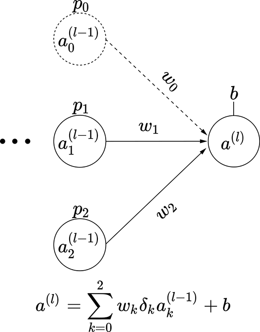
(d) Subnetwork 3: probability P3 = (1−p0 )p1 p2
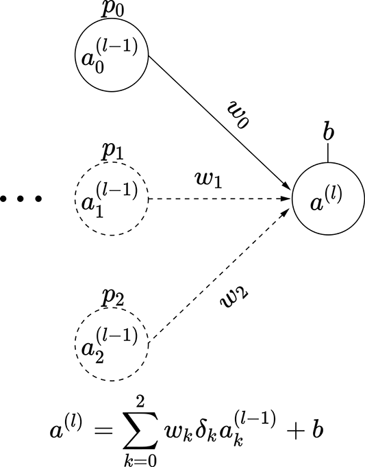
(e) Subnetwork 4: probability P4 = p0 (1−p1) (1−p2)
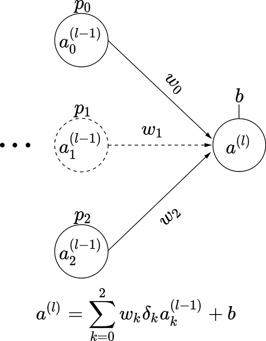
(f) Subnetwork 5: probability P5 = p0 (1−p1) p2
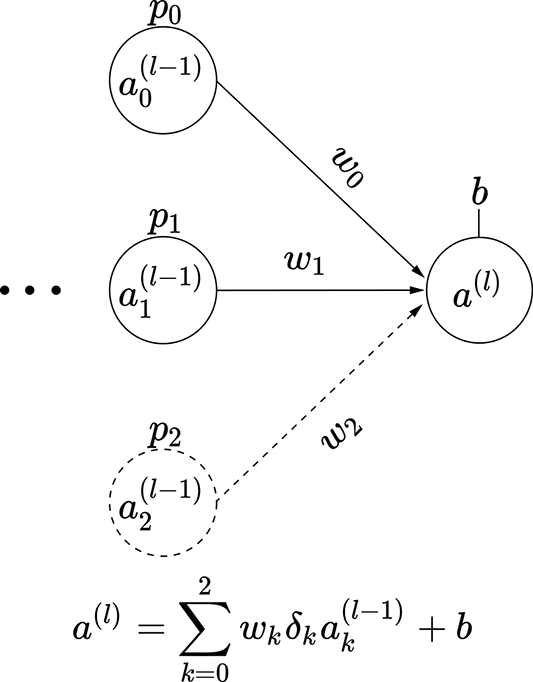
(g) Subnetwork 6: probability P6 = p0 p1 (1−p2)
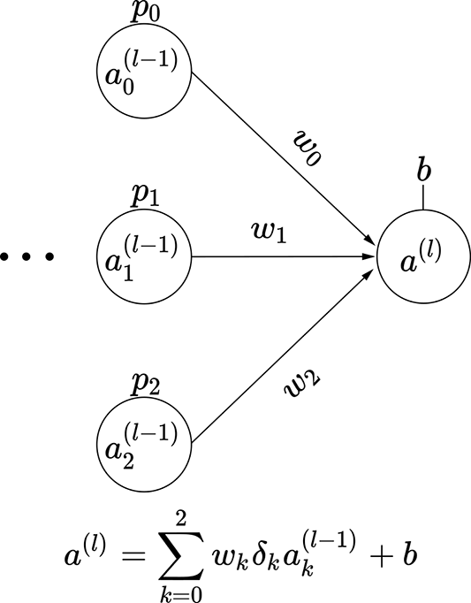
Figure 9.13 Dropout simulates subnetworks: illustrated with a three-node intermediate layer of a neural network. The probability of input node ak(l − 1) being on is p(δk = 1) = pk.
Summary
-
Training is the process by which a neural network identifies the optimal values for its parameters (weights and biases of the individual perceptrons). Training progresses iteratively: in each iteration, we estimate the loss and run an optimization step that updates the parameter values so as to decrease the loss. After doing this many times, we hope to arrive at optimal parameter values.
-
In a supervised neural network, loss quantifies the mismatch between the desired output and the network output over sampled training data instances. The desired output (ground truth) is often estimated via manual effort. Training the neural network essentially identifies the weights and biases of the neural network that minimize the loss.
-
The discrepancy between the ground truth and network output can be expressed in many different ways. Each corresponds to a different loss function. Denoting the ground truth probabilities of all the possible classes given the ith training input
 (i) as a vector ȳ(i) and the network output on the same as y(i),
-
Regression loss takes the L2 norm of the vector difference between the network output and ground-truth vectors and is mathematically expressed as
 .
. -
If the neural network is a classifier, it typically outputs a vector of class probabilities. This means

where pj((i)) is the network estimated probability of the input belonging to class j, and N is the number of possible classes. In general, given an input, a neural network computes per-class scores: the class with the highest score is the predicted class. The scores are unbounded numbers and can be arbitrarily large or small (even negative). The operation converts them into probabilities. If
denotes the score vector, the corresponding softmax vector is
where . The softmax output vector consists of probabilities, meaning they are numbers between 0 and 1 and they sum to 1.
 -
Given the probability of each class, classifiers can employ the cross-entropy loss, which can be expressed as
 .
.
Note that since the ground-truth vector is one-hot, only a single term in this expression survives: the one corresponding to the desired class, denoted j*. The loss becomes the logarithm of the corresponding network output, −log(yj*(i)), and is zero if yj*(i) = 1. This agrees with our expectation: if the network is predicting the GT class with probability 1, there is no loss. -
Since during training, softmax is almost always followed by cross-entropy loss, PyTorch has a combined operator called softmax cross-entropy loss. It is over doing these operations individually because it has better numerical properties.
-
Focal loss tries to tackle the data-imbalance problem by putting more weight on the “hard” examples with higher loss.
-
Hinge loss is another popular loss that becomes zero when the correct class is predicted with the maximum score. Once that criterion is achieved, it no longer tries to improve the relative values of scores.
-
-
Total loss can be obtained by adding the losses from all the individual training data instances. However, this requires us to process all the training data points in every iteration, which is prohibitively expensive. Hence, we sample a subset of training data points to create a minibatch, estimate losses for each input data instance in the minibatch, and add them to obtain an estimate for the total loss. This process is known as stochastic gradient descent (SGD).
-
Optimization is the process of updating the neural network parameters (weights and biases of perceptrons) so as to reduce the loss. We can plot the loss against weights and bias values and obtain a hypersurface defined over the domain of weights and bias values. Our ultimate goal is to reach the bottom (minimum point) of this loss hypersurface. Optimization is geometrically equivalent to moving down the hypersurface to reduce the loss. The steepest descent (toward the nearest minimum) happens along a negative gradient.
-
We can combine several other criteria with the gradient to improve the convergence to the minimum loss value. Each of them results in a different optimization technique:
-
Due to noisy estimations, the local gradient may not always point toward the minimum, but it will have a strong component toward that minimum along with other noisy components. Instead of blindly following the current gradient, we can follow the direction corresponding to a weighted average of the current gradient estimate and the gradient estimate from the previous iteration. This is a recursive process, which effectively means the direction followed at any iteration is a weighted average of the current and all gradient estimates from the beginning of training. Recent gradients are weighted higher, and older gradients are weighed lower. All these gradients have strong components toward the minimum that reinforce each other, while the noisy components point in random directions and tend to cancel each other. Thus the overall weighted sum is a more reliable move toward the minimum. This is called momentum-based gradient descent.
-
A drawback of momentum is that it can result in overshooting the minimum. Nesterov accelerated gradients correct this drawback by calculating gradients via one-step lookahead. If the current update takes us to the other side of the minimum, the gradient will have an opposite direction there. We take a weighted average of the update suggested by momentum-based gradient descent and the gradient at the estimated destination point. If we are far from the minimum, it will be roughly equivalent to momentum-based gradient descent. But if we are about to overshoot the minimum, there will be cancelation, and the update will be smaller than that of the pure momentum case. Thus we reduce the chances of overshooting the minimum.
-
AdaGrad is an optimization technique that imparts additional weight to infrequently changing axes of the loss hypersurface. The Adam optimizer combines many advantages of other optimizers and is often the modern optimizer of choice.
-
-
The principle of Occam’s razor essentially says that among adequate explanations, the simplest one should be preferred. In machine learning, this leads to regularization. There are typically many solutions to the loss-minimization problem. We want to choose the simplest one. Accordingly, we add a penalty for departing from simplicity (regularization loss) to whatever other losses we have. This incentivizes the system to go for the simplest solution. Regularization loss is often the total length of the parameter vector; thus, regularization pushes us toward solutions with smaller absolute values for parameters.
-
Minimizing the loss function without the regularization term is equivalent to the Bayesian maximum likelihood estimation (MLE) technique. On the other hand, minimizing loss with the regularized term is equivalent to maximum a posteriori (MAP) estimation.
-
Overfitting is a phenomenon where the neural network has learned all the nuances of the training data. Since anomalous nuances in training data points are often caused by noise, this leads to worse performance during inferencing. Overfitting is symptomized by great accuracy (low loss) on training data but bad accuracy on test data. It often happens because the network has more expressive power than necessary for the problem and is trying to memorize all nooks and bends of the training data. Regularization mitigates the problem. Another trick is dropout, where we deliberately turn off a random subset of neurons during training iterations. This forces all the neurons to learn to do the job with a reduced set of neurons.